Dynamic mode decomposition is a modern, data-driven modeling technique designed to uncover hidden patterns inside complex time-dependent systems. From fluid flows to financial markets, this method translates high-dimensional measurements into clear, structured representations. By identifying spatial modes and their temporal evolution, it allows researchers to understand how systems change, oscillate, grow, or decay over time.

In today’s era of big data, dynamic mode decomposition has become increasingly valuable because it does not require full knowledge of governing equations. Instead, it learns directly from collected data snapshots. This flexibility makes it highly attractive across engineering, physics, artificial intelligence, and economics, where interpreting system dynamics quickly and efficiently is essential.

Foundations of Dynamic Mode Decomposition

Linear Algebra and Data Structure

At its mathematical core, dynamic mode decomposition relies on linear algebra concepts such as matrices, eigenvalues, and singular value decomposition. The process begins by arranging time-series data into snapshot matrices that represent consecutive measurements of a system. These matrices allow the algorithm to compare how a system transitions from one state to the next.

Singular value decomposition reduces the dimensionality of the dataset while preserving its dominant features. This reduction is crucial because many real-world systems produce extremely high-dimensional data. By focusing on the most influential components, dynamic mode decomposition creates stable and efficient reduced-order models that still capture essential behavior.

Dynamical Systems and the Koopman Perspective

Dynamic mode decomposition is strongly connected to dynamical systems theory, particularly the concept of the Koopman operator. Even when a system behaves nonlinearly, this approach approximates it using linear transformations in a higher-dimensional feature space. This unique perspective enables the analysis of nonlinear phenomena through linear mathematical tools.

By examining eigenvalues derived from the reduced operator, researchers can interpret growth rates, decay rates, and oscillatory frequencies within the system. This spectral insight provides both predictive power and interpretability. As a result, dynamic mode decomposition bridges theoretical mathematics and practical modeling in a highly efficient manner.

The DMD Algorithm Explained

Step-by-Step Computational Process

The algorithm begins by collecting sequential snapshots of a dynamic system. These snapshots are separated into two matrices representing past and future states. The goal is to approximate a linear operator that maps one state to the next. This mapping defines how the system evolves over time.

After applying singular value decomposition to reduce complexity, the algorithm constructs a low-rank approximation of the system operator. Eigenvalues and eigenvectors are then computed to extract dynamic modes. These modes describe recurring spatial structures and their associated temporal behaviors, forming the backbone of the dynamic mode decomposition framework.

Interpreting Modes and Eigenvalues

The output of dynamic mode decomposition consists of spatial modes linked with specific eigenvalues. Each eigenvalue reveals how its corresponding mode behaves, including whether it grows, decays, or oscillates. This detailed insight makes the technique particularly valuable for identifying dominant patterns in complex datasets.

Interpreting these modes allows analysts to reconstruct system behavior and even forecast future states. Because each mode represents a coherent structure, researchers can isolate meaningful features from noisy data. This interpretability is one of the defining strengths of dynamic mode decomposition compared to many black-box machine learning models.

Variants and Extensions of Dynamic Mode Decomposition

Exact and Extended Approaches

dynamic mode decomposition As the method evolved, several enhanced versions were introduced to address specific challenges. Exact DMD improves numerical accuracy and ensures consistent modal extraction. Extended DMD expands the observable space, enabling better representation of nonlinear dynamics using richer functional transformations.

These variations increase flexibility and broaden applicability. In scenarios where standard linear assumptions may fall short, extended formulations allow dynamic mode decomposition to approximate more complicated system behavior while maintaining mathematical clarity and computational efficiency.

Multi-Resolution and Sparsity-Promoting Methods

Multi-resolution DMD decomposes systems across different time scales, making it ideal for analyzing multi-frequency processes such as climate cycles or mechanical vibrations. This layered analysis reveals hidden dynamics that may otherwise remain undetected in traditional implementations.

Sparsity-promoting methods focus on selecting the most relevant modes while discarding redundant ones. By reducing overfitting and improving clarity, these approaches enhance the reliability of dynamic mode decomposition in large or noisy datasets. Such refinements continue to strengthen the method’s role in advanced data analysis.

Applications of Dynamic Mode Decomposition

Engineering and Fluid Dynamics

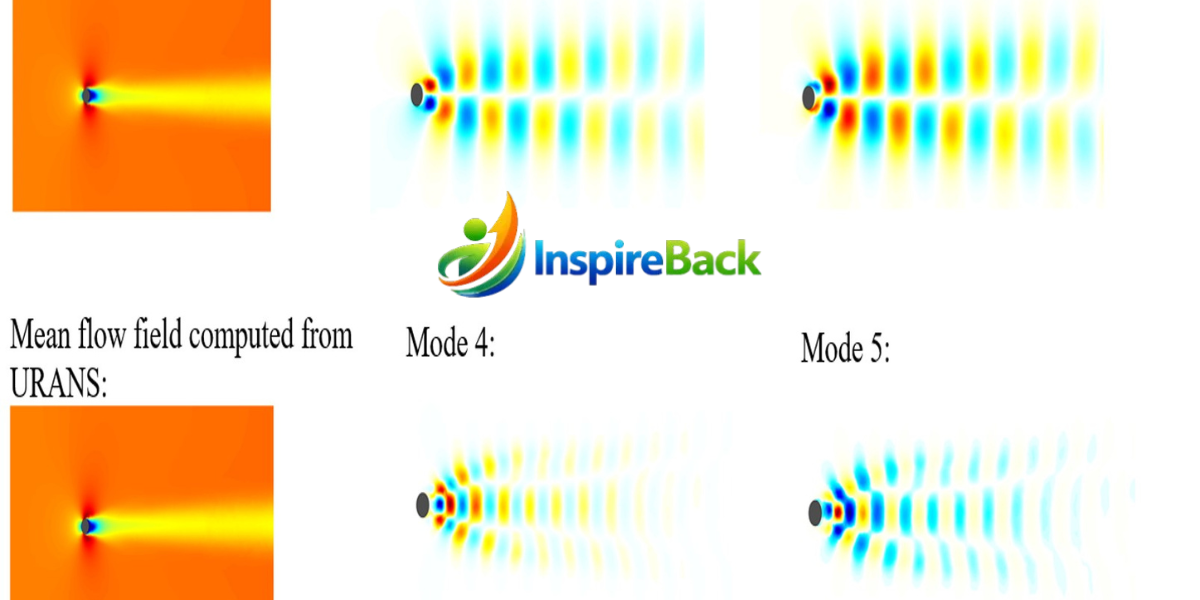
Dynamic mode decomposition was originally popularized in fluid mechanics, where it helps identify coherent flow structures within turbulent systems. Engineers use it to simplify computational simulations and optimize aerodynamic performance. Its ability to extract dominant flow patterns makes it indispensable in aerospace and mechanical engineering.

In industrial settings, the technique supports fault detection and system monitoring. By analyzing vibration data or pressure fluctuations, engineers can detect anomalies before failures occur. This predictive capability significantly improves safety, efficiency, and operational reliability.

Finance, Neuroscience, and Data Science

In finance, dynamic mode decomposition assists in analyzing time-series data such as stock prices or economic indicators. It helps identify recurring cycles and market regimes, offering insights into risk modeling and forecasting. Its structured modal interpretation makes it attractive to quantitative analysts.

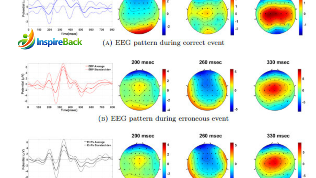
In neuroscience and biomedical engineering, researchers apply the technique to brain signal analysis and physiological data modeling. It enables the identification of rhythmic activity and dynamic patterns in neural recordings. Across data science disciplines, the method supports feature extraction, dimensionality reduction, and system forecasting tasks.

Comparison with Other Analytical Techniques

Dynamic mode decomposition is often compared with principal component analysis and proper orthogonal decomposition. While those methods focus primarily on spatial variance or energy content, DMD emphasizes temporal evolution. This distinction makes it especially useful for predictive modeling and understanding dynamic behavior.

Compared to deep learning models, dynamic mode decomposition offers greater interpretability and lower computational requirements. Neural networks may require extensive training data and tuning, whereas DMD provides immediate spectral insights from structured linear algebra operations. This balance between transparency and performance explains its growing popularity.

Advantages and Practical Considerations

One major advantage of dynamic mode decomposition is its equation-free framework. It operates purely on data, making it ideal for systems where governing equations are unknown or difficult to derive. Its reduced-order models are computationally efficient and suitable for real-time analysis.

However, careful implementation is necessary to manage sensitivity to noise and rank selection. Preprocessing data and choosing appropriate truncation levels during singular value decomposition are essential for accurate results. When applied thoughtfully, dynamic mode decomposition becomes a powerful and reliable analytical tool.

Conclusion

Dynamic mode decomposition represents a transformative approach to understanding complex dynamical systems. By combining linear algebra with data-driven modeling, it extracts coherent structures that reveal how systems evolve over time. Its interpretability and computational efficiency distinguish it from many traditional and modern analytical techniques.

As industries continue to generate massive time-dependent datasets, the relevance of dynamic mode decomposition will only grow. From engineering to finance and neuroscience, its adaptable framework provides clarity in complexity. For researchers and professionals seeking deeper insight into dynamic systems, this method remains an essential and forward-looking solution.

Frequently Asked Questions

What is dynamic mode decomposition used for?

Dynamic mode decomposition is used to analyze time-series data, identify dominant patterns, and build reduced-order predictive models for complex systems.

Is dynamic mode decomposition suitable for nonlinear systems?

Yes, extended versions approximate nonlinear dynamics through higher-dimensional linear representations inspired by Koopman theory.

How does dynamic mode decomposition differ from PCA?

Unlike PCA, which focuses on spatial variance, dynamic mode decomposition captures both spatial structures and their temporal evolution.

Can dynamic mode decomposition forecast future behavior?

Yes, by analyzing eigenvalues and temporal modes, it can reconstruct and predict system states over time.

What software supports dynamic mode decomposition?

It is commonly implemented in Python and MATLAB using scientific computing libraries and open-source packages.

Also Read: yukon license plate